Last time, I showed that the variance among siblings is always half as much as their parent’s generation’s variance. And this doesn’t depend on assortative mating — it’s always true no matter how similar couples are.
However, a commenter pointed out that assortative mating will increase the variance of the kid’s generation. In math:
\mathbb{V}(Siblings) = \frac{1}{2}\mathbb{V}(Parents)\mathbb{V}(Kids) \geq \mathbb{V}(Parents)\implies \mathbb{V}(Siblings) \leq \frac{1}{2} \mathbb{V}(Kids)It turned out on simulation that, in perfect assortative mating,
\mathbb{V}(Siblings) = \frac{1}{3}\mathbb{V}(Kids)So at intermediate levels, the variance of siblings will be between 33% and 50% of the variance of their peers.
SIZE = 1000
ps = np.random.normal(.5,.15,SIZE)
ps[ps > 1] = .999
ps[ps < 0] = 0.01
fifties = [0.5 for i in range(SIZE)]

NUM_FAMS = 250
vars = []
parents = np.zeros((NUM_FAMS*2, SIZE))
all = np.zeros((NUM_FAMS*NUM_KIDS, SIZE))
for _ in range(NUM_FAMS):
    print(_/NUM_FAMS, end="\r")
    NUM_KIDS = 100
    m1 = np.random.binomial(1, ps)
    m2 = np.random.binomial(1, ps)
    f1 = np.random.binomial(1, ps)
    f2 = np.random.binomial(1, ps)
    parents[2*_] = m1 + m2
    parents[(2*_)+1] = m1 + m2
    kids = np.zeros((NUM_KIDS, SIZE))  # row: kid genome. col: genes
    for i in range(NUM_KIDS):
        samples = np.random.binomial(1, fifties)
        samples2 = np.random.binomial(1, fifties)
        kid1 = np.where(samples == 0, m1, m2)  # same as kid1 = np.array([m1[idx] for idx in range(SIZE) if (samples[idx] == 0) else (m2[idx]) ]) but written in C
        kid2 = np.where(samples2 == 0, m1, m2)  # make m1,m2 for perfect assortative mating, f1,f2 for random mating
        kids[i] = kid1 + kid2
    # Add all of the kids matrix to 'all'
    varst = np.var(kids, axis=0)
    vars.append( np.sum(varst))
    all[_*NUM_KIDS:(_+1)*NUM_KIDS] = kids  # Adding the kids to 'all'

# Compute the variance of the kids
kids_var = np.var(all, axis=0)
kids_var_sum = np.sum(kids_var)
vars.append(kids_var_sum)

# Convert vars to a numpy array
vars = np.array(vars)

# Compute the variance of the parents
parentvarl = np.var(parents, axis=0)
parentvar = np.sum(parentvarl)
sibvar = vars.mean()
print("Variance of kids:", kids_var_sum)
print("Variance of parents:", parentvar)
print('ratio', kids_var_sum/parentvar)
print(sibvar/kids_var_sum)
'''
OUTPUT:
Variance of kids: 682.1616028943927
Variance of parents: 455.08419200000003
ratio 1.498978902994707
0.3321545100723841
'''
Why does this happen? Each allele is the sum of the binary values at two loci:
A_i = L_{i,1} + L_{i,2}and each gene score is the sum of all the allele values. So:
\mathbb{V}(Kids) = \frac{3}{2}\mathbb{V}(Parents) \implies \sum_i \mathbb{V}(A_i)_{Kids} = \frac{3}{2} \sum_i \mathbb{V}(A_i)_{Parents}\mathbb{V}(A_i)_{Kids} = \frac{3}{2} \mathbb{V}(A_i)_{Parents} \implies \mathbb{V}(L_{i,1}) + \mathbb{V}(L_{i,2}) + 2Cov(L_{i,1}, L_{i,2}) = \frac{3}{2}( \mathbb{V}(L_{i,1}) + \mathbb{V}(L_{i,2}) )This is because the covariance term is 0 in the parental generation, as the parents were assumed to be in Hardy-Weinberg equilibrium. We simplify to:
Cov(L_{i,1}, L_{i,2})_{kids} = \frac{1}{4}( \mathbb{V}(L_{i,1}) + \mathbb{V}(L_{i,2}) ) = \frac{1}{4} (pq + pq) = \frac{1}{2}pqUnder perfect assortative mating, this equation is true.
Cov(L_{i,1}, L_{i,2}) = \mathbb{E}[L_{i,1}L_{i,2}] - \mathbb{E}[L_{i,1}]\mathbb{E}[L_{i,2}] = \mathbb{P}(11) - p^2It turns out that
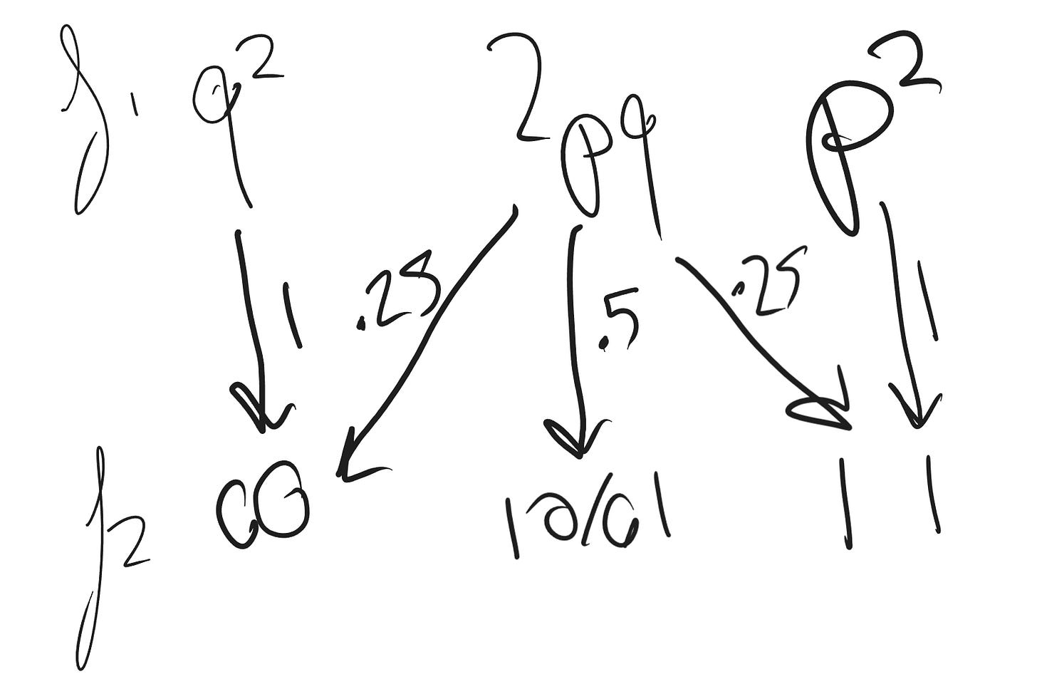
\mathbb{P}(11) = p^2 + \frac{1}{2}pqSo both sides of the equation are the same.
Why the last equation? Under perfect assortative mating, each homozygote always produces a batch of all homozygotes. But heterozygotes produce half heterozygotes and one quarter homozygotes of each type.