Demystifying Regression to the Mean

I have been asked to write about regression to the mean by some readers. Previous articles provided simulations and intuitions — I will add onto this some mathematical concepts as well as some more intuitions behind these.

Variance Decomposition of IQ

The other articles’ simulations were based on decomposing IQ into two sources: additive genetics and everything else, which we can call the “broad environment.”

Mathematically, this looks like this:

p_i = hg_i + (\sqrt{1-h^2})e_i

Where p is phenotype, g is additive gene score, and e is broad environment. Here, each of the random variables is defined as having a mean of 0 and a variance of 1. The constant terms control how much of the resulting phenotype variance each component explains.

Taking the variance of both sides,

\mathbb{V}[p_i] = \mathbb{V}[hg_i + (\sqrt{1-h^2})e_i] \implies 1 = h^2 + (1-h^2) = 1

Assuming no covarance between gene score and broad environment. h^2 is familiar — it is the phenotypic “variance explained” by genetics, a.k.a the heritability. Our second equation shows why the coefficient in front of g_i becomes h when h^2 is used as g_i’s “variance explained”.

Conditional Expectation Functions

To analyze what happens when we select people based on phenotype, we need to understand conditional expectation functions. If we allow g to be random, we can write the following:

\mathbb{E}[p_i|g_i] = hg_i + \mathbb{E}[(\sqrt{1-h^2})e_i] = h g_i

This means if we select on genotype, we expect an above average phenotype as well. But we’re selecting on phenotype, so we need the CEFs given p of g and e.

Assuming no covariance between e and g, we get

g_i = hp_i + \epsilon_i \implies \mathbb{E}[g_i | p_i] = h p_i

and

e_i = (\sqrt{1-h^2})p_i  + \epsilon_i \implies \mathbb{E}[e_i 
| p_i] = (\sqrt{1-h^2})p_i

Using these functions, if we let h^2 = 1/2, and if we select a trillion people with an average IQ of 1 SD, then their average environment and genotype will both be about 0.70 SD.

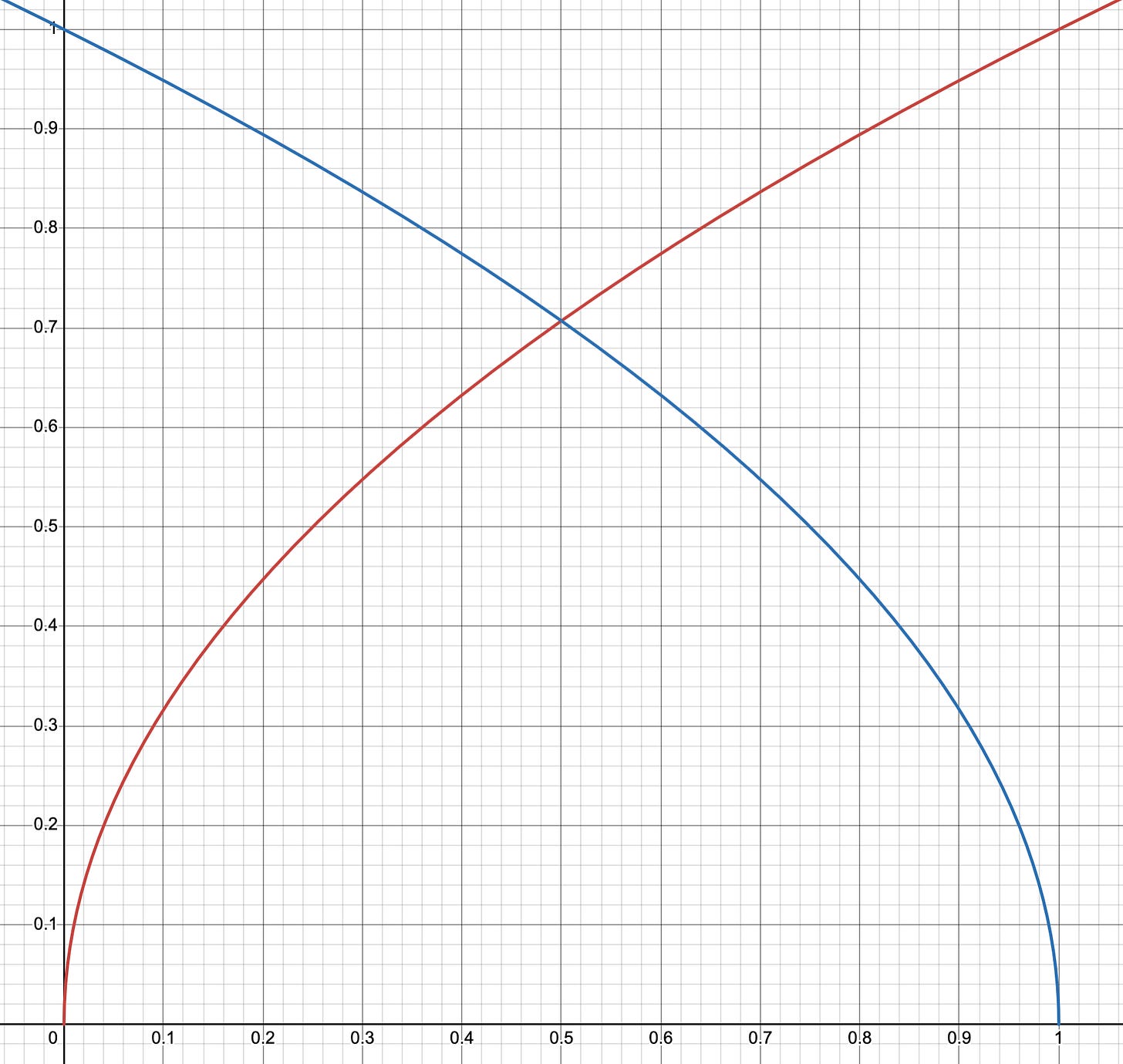
As you can see, when selecting on something, associated correlate means are always less extreme. Mathematically, this is due to the Cauchy-Schwarz inequality, which bounds correlations between -1 and 1.

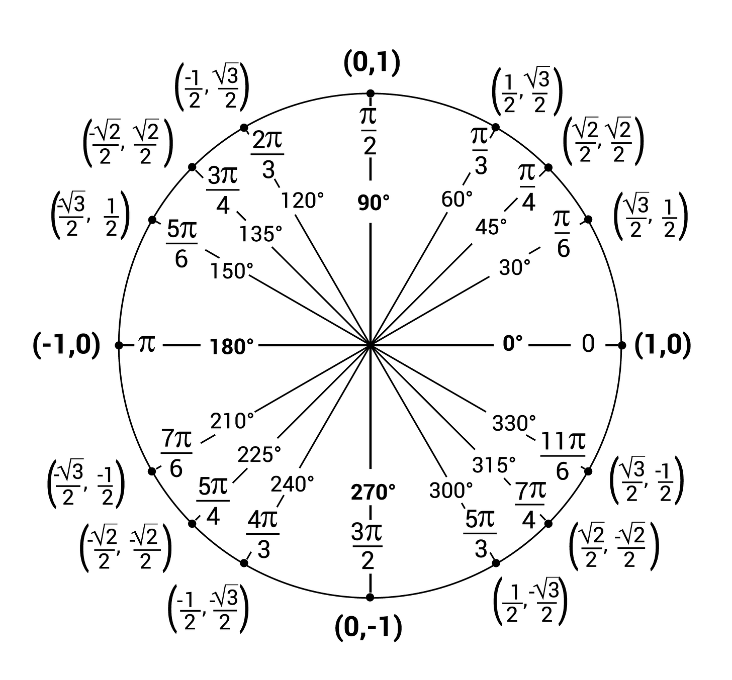
What is the intuition for this? We can derive it from 2D or 3D linear algebra. Once data has been standarzed, the correlation between two samples is the same as the projection of one unit vector onto another. The Cauchy-Schwarz inequality also tells us this is between -1 and 1.

|<x,y>| \: \leq ||x|| \: ||y|| \implies |<u_1,u_2>| \leq 1

Why? You can draw vector projection in 2D. Projection finds the point on one vector’s span that minimizes the distance to the projected vector. Projections are always orthogonal. If you project a unit vector onto a unit vector, think about what you get.

If you let your projected onto vector be [1,0], and vary your projectee but keep it unit length, you get the unit circle, where the cosine/x coordinate is the projection length. You can confirm visually that it is always between -1 and 1.

More intuitively, imagine walking along an arbitrary path for 1 mile. Then you wonder, how far east did you move from your starting position? If you went north or south, or, it’s 0 miles. If you went west, it’s -1 miles. If you went directly east, it’s 1 mile. If you went northeast, it’s sqrt(2)/2 =~ 0.70. It can’t be more than 1 because you only moved 1 mile.

Back to random variables, you standarize everything before analysis so it’s all 1 SD and 0 mean. If you have a group with 1 SD IQ, how is it possible to have a 1 SD average gene score? This would imply that phenotype is the exact same as genotype. When you measure one, you measuring the other, so that when you standardize the data, you get perfect correspondence. Anything less than perfect correspondence will decrease the correlation, by definition.

Immigrants and Quantitative Genetics

It’s more of a finding of quantitative genetics and less of a consequence of linear regression that inter-generation regression to the mean happens once. If you have a closed off, selected breeding group chosen from a large population under no evolutionary pressure, and environment is strictly independent from genes, then the average standarized gene score of the next generation will be the same as the average gene score of the breeding group, while the average environment will be the broader environmental mean.

Let’s think back to our group from before: they had 1 SD IQs on average, which gave them 0.70 SD environments and genotypes. Their offspring have an average genotype of 0.70 SD and an average environment of 0 SD, giving them IQs of 0.7 * 0.7 = h^2, or 0.5 SD.

They breed again in the same place. What happens? The next generation has a 0.70 SD genotype and a 0 SD environment, giving them IQs of 0.7 * 0.7 = h^2, or 0.5 SD. This generation breeds again. What happens? … etc.

Many people intuit that gene scores themselves regress to the mean when that is not the case. First, the average parental midpoint under random mating is

\mathbb{E}[\frac{g_m + g_f}{2}] = \frac{1}{2}(\mathbb{E}[g_m] + \mathbb{E}[g_f]) = \mathbb{E}[g]

Now consider a single loci. The parental midpoint at that loci is

\bar{f} = \frac{1}{2}((X_{m,1} + X_{m,2}) + (X_{f,1} + X_{f,2}))

The expected value for the child’s X is:

\mathbb{E}[X_c] = \frac{1}{4}(X_{m,1} + X_{f,1}) + \frac{1}{4}(X_{m,1} + X_{f,2}) + \frac{1}{4}(X_{m,2} + X_{f,1}) + \frac{1}{4}(X_{m,2} + X_{f,2})

And this clearly multiplies out to be the same as the parental midpoint at a loci. Putting it all together (left as an exercise for the reader — remember the gene score is a weighted sum of loci values), the average child will have a gene score equal to the average adult.